MODEL CALIBRATION

At the core of modeling lies our ability to estimate the values of the model's parameters.
This process is known as parameter estimation, and it relies on a method called optimization.
During an optimization process, we systematically adjust the model parameters until the difference between the model's predictions and the experimental data points is minimized.

In the interactive example below, you can experiment by changing the parameter of a linear model and observing how it affects the distance between the model's line and the experimental data points.
There are several ways to quantify this distance. One commonly used metric is the root mean squared error (RMSE), defined as:

Where:

• $y_i^e$ is the experimental (observed) value
• $y_i$ is the value predicted by the model
• n is the number of data points

Now consider: how does changing the model parameter affect the RMSE?

As you can see, there is a minimum in the function that relates RMSE to the model parameter.
The value of the parameter (in this case, a) that produces the lowest RMSE is the optimal parameter — the one that best fits the data.

Well done! You've just completed your first manual optimization task of the course!

MODEL EXAMPLE: The HR_max = 220 − Age MODEL

The formula HR_max = 220 − Age is one of the most well-known and commonly used methods for estimating an individual's maximum heart rate (HR_max). However, its popularity stands in contrast to its empirical limitations and historical origins, which are surprisingly informal.

Despite its limitations, the formula remains in use due to its simplicity. However, as sport scientists, it's essential to understand its shortcomings:

• It tends to underestimate HR_max in older adults
• It often overestimates HR_max in younger individuals
• The typical error margin can be as high as ±10–12 bpm, which is significant when prescribing training intensities

Clearly, this is a parametric model that could benefit from being calibrated or tuned to specific populations—athletes, clinical groups, children, women, or elderly subjects.

To overcome the issues with the 220 − Age model, researchers have proposed improved formulas based on larger and more diverse datasets.

✅ Tanaka et al. (2001): General Population

• Based on a meta-analysis of 351 studies (~18,000 subjects)
• Includes both males and females, across various age groups
• Provides a lower standard error than the 220 − Age model
• Widely adopted in both sports science and clinical applications

✅ Gulati et al. (2010): Female-Specific Model

• Derived from a large cohort of 5,437 healthy women
• Addresses the known sex differences in cardiovascular physiology
• Particularly useful for female athlete training and cardiac rehabilitation

When designing training plans or assessing cardiovascular capacity, we must remember that no single model fits all. Variability exists between individuals and across groups, and models must be evaluated for their applicability, assumptions, and predictive accuracy.

As a sport scientist, always ask:

• What population was the model derived from?
• How large and diverse was the dataset?
• What is the typical error margin?
• Are the parameters relevant for your specific context?

Try yourself to tune the parameters and minimise the RMSE. Is the RMSE equally minimised for both females and males for the same parameters? What does this mean?

Practical Implementation: Model Calibration Tools

Now that you understand the optimization principles, let's explore how to implement these concepts using practical tools. In this course, you'll primarily work with spreadsheets (Excel and Google Sheets), but we'll also show you when and why you might need more advanced programming approaches.

Excel: Your Primary Tool

Method 1: Trendline (Quick but Limited)

Excel's built-in trendline feature provides the simplest approach:

1. Plot your experimental data as a scatter chart
2. Right-click on data points → "Add Trendline"
3. Choose from: Linear, Exponential, Logarithmic, Polynomial, Power, Moving Average
4. Select "Display Equation" and "Display R-squared"
5. Excel automatically optimizes the parameters for you

Limitation: You're restricted to Excel's predefined functions. Custom equations like the Hill muscle model or Critical Power relationship require a different approach.

Method 2: Solver Add-on (Full Flexibility)

For any custom model equation, follow this systematic approach:

1. Set up your model: Create columns for:

   • Experimental data (x, y)
   • Parameter cells (clearly labeled)
   • Model predictions using your equation

2. Calculate residuals: In a new column, compute: =(Experimental - Predicted)^2

3. Compute RMSE: Use =SQRT(AVERAGE(residuals_range))

4. Enable Solver:

   • Go to File → Options → Add-ins → Excel Add-ins
   • Check "Solver Add-in" → OK

5. Run optimization: Data tab → Solver

   • Objective: Select your RMSE cell (set to minimize)
   • Variable cells: Select your parameter cells
   • Click Solve: Excel finds optimal parameters automatically!

Example: For HR_max = a × Age + b, you'd have parameter cells for 'a' and 'b', and Solver would minimize RMSE by adjusting these values to best fit your data.

Google Sheets: Similar Capabilities

Trendline: Works identically to Excel—same options, same limitations.

Solver Workaround: Google Sheets lacks a built-in Solver, but you have alternatives:

• Goal Seek: Data → Goal Seek (limited to single-parameter optimization)
• Google Apps Script: Write custom optimization routines
• Add-ons: Search "Solver" in the Google Workspace Marketplace for third-party solutions

I found two add-ons: the Optimization Solver and OpenSolver. I only tested the second one. I do not think these tools are ready yet. I found it very hard to solve very basic problems with them.

When Programming Becomes Necessary

As your models become more sophisticated, spreadsheets reach their limits. Here are practical examples:

Python Example: Critical Power Model

import numpy as np
from scipy.optimize import minimize

# Experimental data: time (s) and power (W)
time_data = np.array([180, 300, 600, 1200])
power_data = np.array([400, 350, 300, 275])

def critical_power_model(params, t):
    CP, W_prime = params
    return W_prime / t + CP

def objective_function(params):
    predicted = critical_power_model(params, time_data)
    rmse = np.sqrt(np.mean((power_data - predicted)**2))
    return rmse

# Initial parameter guess
initial_guess = [250, 15000]  # CP=250W, W'=15000J

# Optimization
result = minimize(objective_function, initial_guess)
CP_opt, W_prime_opt = result.x

print(f"Optimal CP: {CP_opt:.1f} W")
print(f"Optimal W': {W_prime_opt:.0f} J")
print(f"RMSE: {result.fun:.2f} W")

MATLAB Example: VO₂ Kinetics

% VO2 kinetics model: VO2(t) = A + Delta*(1 - exp(-t/tau))
vo2_model = @(p, t) p(1) + p(2) * (1 - exp(-t / p(3)));

% Objective function (RMSE)
objective = @(p) sqrt(mean((vo2_exp - vo2_model(p, time)).^2));

% Optimization
p_opt = fminsearch(objective, [1.0, 2.0, 30.0]);

fprintf('Optimal parameters: A=%.2f, Delta=%.2f, tau=%.1f\n', p_opt);

When to Move Beyond Spreadsheets

Complex Models: Multi-parameter differential equations, nested functions

Large Datasets: Thousands of data points that overwhelm Excel

Advanced Algorithms: Constraints, bounds, specialized optimization methods

Automation: Batch processing multiple athletes or conditions

Reproducibility: Version control and automated analysis pipelines

The Learning Progression: Start with Excel to grasp the fundamental concepts of optimization and RMSE minimization. As your models become more sophisticated and your datasets larger, programming languages provide the flexibility and power needed for advanced analysis.

Remember: The mathematical principles remain constant—whether you're using Excel's Solver or Python's scipy.optimize, you're still minimizing RMSE by adjusting parameters. Only the implementation tool changes.

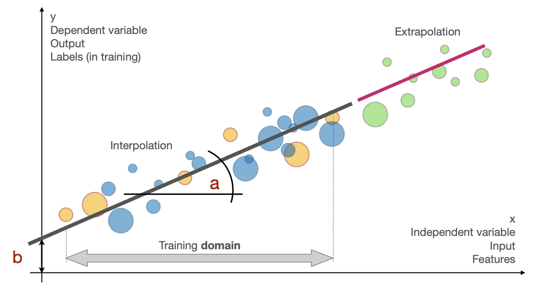
Interpolation vs. extrapolation

One of the most critical distinctions in model application is between interpolation (making predictions within the range of observed data) and extrapolation (making predictions beyond the observed range). This difference becomes dramatically apparent when examining Olympic 100-meter sprint records over time.

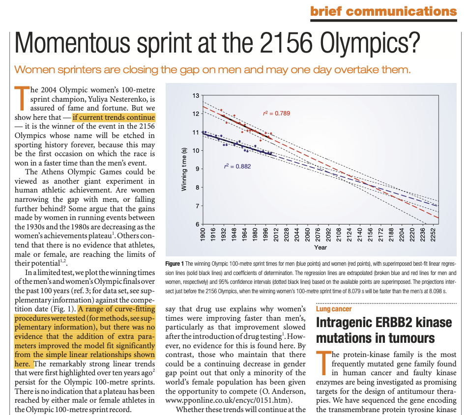
Even in the most prestigious journals, modeling approaches can lead to misleading result interpretations. The figure above, published in Nature (2004), demonstrates how extrapolation of Olympic sprint trends can produce controversial predictions—suggesting that women would eventually outperform men in 100-meter sprints by 2156.

The interactive chart below uses the same Olympic data from the original paper, but presents a careful revisitation of the analysis. We show Olympic winning times from the early 1900s to present, with linear regression models fitted to both men's and women's data. The models extend their predictions to the year 2252—more than two centuries into the future.

What do these models predict? By 2252, the linear extrapolation suggests men's times would approach zero seconds, while women's times would become negative—physically impossible outcomes that highlight the fundamental problem with extrapolation.

When we fit models to historical data (roughly 1900-2020), we capture trends that may be valid within that time period. However, extrapolation assumes these trends continue indefinitely, ignoring several crucial factors:

Physical limitations: Human sprint performance cannot improve indefinitely. Physiological constraints—muscle fiber types, energy systems, biomechanical efficiency—impose absolute limits that mathematical models ignore.

Environmental and social changes: The dramatic improvement in women's performance reflects historical factors like increased participation, better training, and social acceptance of women's athletics. These improvements naturally slow as conditions reach parity.

Non-linear effects: The quadratic model (available via checkbox) shows how performance improvements may plateau over time, capturing the concept of diminishing returns more realistically than linear extrapolation.

Technological and regulatory boundaries: Track surfaces, shoe technology, altitude effects, and anti-doping measures all influence performance in ways that historical models cannot anticipate.

This example illustrates why extrapolation requires extreme caution. While interpolation leverages observed relationships within known boundaries, extrapolation ventures into unknown territory where our model's assumptions may no longer hold. The further we extrapolate, the less reliable our predictions become.

Overfitting: the hidden cost of complexity

When building models, it's tempting to believe that more complex models always provide better predictions. After all, if we can achieve a higher R² (coefficient of determination) by adding more parameters, shouldn't we do so? This logic leads us into one of the most common pitfalls in modeling: overfitting.

The interactive chart below demonstrates overfitting using actual chicken growth data. We have only 5 data points representing weight measurements over time, and we can fit increasingly complex polynomial models:

• Linear Model: $\mathrm{Weight} = a_1 \cdot \mathrm{Age} + a_0$ (2 parameters)
• Quadratic Model: $\mathrm{Weight} = a_2 \cdot \mathrm{Age}^2 + a_1 \cdot \mathrm{Age} + a_0$ (3 parameters)
• Cubic Model: $\mathrm{Weight} = a_3 \cdot \mathrm{Age}^3 + a_2 \cdot \mathrm{Age}^2 + a_1 \cdot \mathrm{Age} + a_0$ (4 parameters)
• Quartic Model: $\mathrm{Weight} = a_4 \cdot \mathrm{Age}^4 + ... + a_0$ (5 parameters)

As you switch between models, observe these key patterns:

1. R² increases with model complexity—the quartic model (5 parameters) fits all 5 data points perfectly (R² = 1.000)
2. Predictions at 18 days become increasingly unrealistic with higher-order polynomials
3. The quartic model produces the best fit to the training data but likely the worst predictions for new data

When we have 5 data points and 5 parameters (quartic model), we can fit the training data perfectly, but this creates several problems:

• No degrees of freedom: We cannot assess model validity when parameters equal data points
• Poor generalization: The model memorizes training data rather than learning underlying patterns
• Unrealistic extrapolation: High-order polynomials often produce biologically implausible predictions
• Increased sensitivity: Small changes in data can dramatically alter the model

This illustrates the fundamental bias-variance tradeoff: simple models (linear) may have higher bias (systematic error) but lower variance (sensitivity to data changes), while complex models (quartic) may have lower bias on training data but higher variance and poor generalization.

Prefer simpler models when they provide reasonable fit. Consider biological plausibility of predictions. Reserve complexity for when additional parameters are truly justified. Validate predictions on independent data whenever possible.

The linear model may have the lowest R², but it provides the most interpretable, stable, and generalizable relationship between chicken age and weight.

Checkout

Well done, you were able to complete the second module of this course.