DYNAMIC SYSTEMS

Static vs. Dynamic. A dynamic model accounts for time-dependent changes in the state of a system, while a static (or steady-state) model assumes the system is in equilibrium and does not vary over time—in other words, it is time-invariant.

Dynamic models are typically represented using differential equations. In mathematics, a differential equation relates one or more unknown functions to their derivatives. A derivative is a fundamental concept that quantifies how a function changes in response to changes in its input.

In our case, we are interested in how a variable evolves over time. This means we are specifically concerned with the time derivative of a variable. We write the derivative term as:

This is read as: "the derivative of y with respect to time (t)." Do not worry too much about the notation or mathematics just yet. The important takeaway is that differential equations, those involving derivatives, help us describe how systems change over time, and thus are key to building dynamic models.

For example, a simple model such as:

describes a system where a property (y) increases at a constant rate of 3.

However, one of the most important differential equations in sport science is:

This equation describes a system that reacts exponentially to changes in the input (x(t)). The parameter $\tau$ is the time constant of the system—something we already encountered in Module 3! This equation is one of the most versatile equations in your modelling toolbox 🛠️, believe me. If you get the behaviour of these equations, you can model a wide range of systems, such as: the oxygen consumption dynamics during generic exercise, the supercompensation principle and Banister model, the exponentially weighted moving averages, a resistance-capacitance circuit, and on and on and on.

I ORDER DYNAMIC SYSTEMS

We introduce here the first and second order dynamic models.

The first-order will let you understand the importance of the time-characteristics of these systems. The second-order will let you understand the importance of the inertia, stiffness, and damping of these systems.

The VO₂ Kinetics Model (Dynamic Version)

It is highly recommended to review the static version of the VO₂ model in Module 3 before approaching this dynamic version.

The simplest dynamic formulation of the VO₂ kinetics model is:

This equation describes how the actual oxygen uptake $VO_2(t)$ responds over time to a steady-state target $VO_{2SS}(t)$.

The steady-state oxygen uptake is defined as:

Where:

• $P(t)$ is the power output at time $t$
• $\epsilon$ is the oxygen cost per unit of power (e.g., in mL·W⁻¹·min⁻¹)
• $VO_{2RES}$ is the resting or baseline oxygen consumption

Substituting into the first equation, we get:

Here, you can recognize the derivative operator (rate of change) and the time constant $\tau$, which governs how fast the VO₂ adapts.

To implement this model in a spreadsheet or software, we approximate the derivative using a finite difference method:

Substituting into the dynamic equation:

Now solve for $VO_{2,k+1}$:

This recursive equation lets you compute oxygen uptake step-by-step over time based on power data. This dynamic model allows you to simulate the transient response of oxygen consumption during exercise. It's especially useful for interval training or transitions between work rates. Once implemented in a spreadsheet, you can model and visualize how VO₂ behaves in response to different power profiles over time.

II ORDER DYNAMIC SYSTEMS

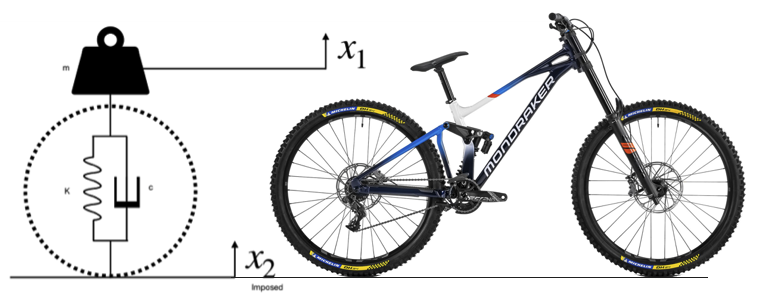
The mass-spring-damping system

One of the main reasons we introduce second-order dynamic models in sports science is because they naturally derive from Newton's second law of motion — the foundation of classical mechanics. You may already be familiar with the general form of this law:

This tells us that an object with mass $m$ will experience an acceleration $a(t)$ that is proportional to the sum of the n external forces F acting on it. Since acceleration is the second derivative of position, we can rewrite this more formally as:

So Newton's law becomes:

In many physical systems, especially those involving movement or impact, we observe three key mechanical properties: inertia, stiffness, and damping. These are particularly relevant in sports settings — for example in the dynamics of skis, rackets, bicycles, and other equipment.

Each of these effects can be captured by a parameter in the classic mass-spring-damper system:

• Inertia is represented by the mass m.
• Stiffness corresponds to a restoring force proportional to the displacement x.
• Damping corresponds to a resistive force proportional to velocity v.

A typical equation of motion for such a system — where a mass is connected to the ground through a spring and a damper — is:

Here, F(t) is a single generic external force applied to the system.
This type of equation is useful when modeling human biomechanics, such as during running, or in this case, for a mountain bike suspension system. In that system, changes in ground elevation drive corresponding changes in the rider's vertical position.

Let's define:

• $x_1$: the vertical position of the rider (the mass),
• $x_2$: the position of the ground (known and imposed),
• K: stiffness of the suspension,
• C: damping coefficient,
• L₀: the equilibrium length of the suspension.

The forces acting on the rider include:

• Spring force: depends on displacement between rider and ground,
• Damping force: depends on the relative velocity between rider and ground,
• Gravity: acts downward on the rider's mass.

We write the equation of motion as:

Rearranging for acceleration:

To use this model in a spreadsheet or code, we discretize the time derivative using a finite difference approximation:

Substituting this into the equation:

And solving for $v_{1,k+1}$:

Since $x_2$ is imposed by the terrain, we can compute $v_2$ directly from it. Then, starting from an initial condition for $x_1$ and $v_1$ at time step k = 0, we can simulate the system step-by-step.

Try it yourself!
Use the sliders to adjust the parameters and see how the model responds to changes in mass, stiffness, damping, or terrain input.

Equation of Motion for Locomotor Sports

Equation of motion, the second-order differential equations introduced previously, form the basis for modeling the dynamics of many locomotor sports such as cycling, cross-country skiing, and running.

In cycling, the primary forces acting on the system (cyclist and bicycle) are:

• $F_P(t)$: Propulsive force generated by the cyclist
• $F_W(t)$: Aerodynamic drag
• $F_R(t)$: Rolling resistance
• $F_G(t)$: Gravitational force due to slope

The dynamic model becomes:

In cycling, we usually monitor effort and performance through power, not force. Power is defined as the product of force and velocity:

Multiplying both sides of the equation of motion by $v(t)$ gives:

This equation expresses how the power produced by the cyclist is used to accelerate the system and overcome resistive forces.

We now replace each force on the right-hand side with its physical expression:

Where:

• $\rho$ is the air density
• $C_{DA}$ is the aerodynamic drag coefficient times frontal area
• $C_{rr}$ is the coefficient of rolling resistance
• $\beta$ is the road gradient (in radians)
• $g$ is gravitational acceleration (9.81 m/s²)

To use this model in a spreadsheet or in code, we discretize the time derivative using a finite difference approximation:

Substituting into the equation:

Solving for $v_{k+1}$:

And of course we do the same to find the distance:

These recursive equations allows you to compute the velocity and distance at the next time step, based on the power input and environmental parameters.

This dynamic model based on Newton's second law gives you a useful tool for simulating motion in sports like cycling. By using power instead of force and discretizing the equations, you can build accurate performance simulations in spreadsheets or programming environments.

Checkout

Well done, you were able to complete the fourth module of this course.