AI models

In Module 4, we fed power into dynamic modelsM4 to predict how VO₂ and cycling speed change over time; here we change the structure of the model, not the way we think about it.

When it comes to Artificial Intelligence (AI), the best-known model structure is the neural network.
We introduce it here by building on the modeling principles you've studied so far, especially inputs, outputs, parameters, and optimization.

A neural network is a sequence of mathematical operations that transforms inputs into outputs, with the aim of reproducing or predicting observed data.
The simplest unit within a neural network is the neuron.

A basic type of neuron, called a perceptron, has two parameters:

• a weight (w) that scales (multiplies) the input
• a bias (b) that shifts (adds to) the result

Weight and bias alone compute $w \cdot x + b$: a straight line, which is exactly the model we fit with linear regression.

What a neuron adds is an activation function, applied to that result before it is passed on. The one we use here is the ReLU (Rectified Linear Unit), $\mathrm{ReLU}(z) = \max(0, z)$: it passes positive values unchanged and sets negative ones to zero.
This matters: without an activation, stacking neurons still gives a linear model, equivalent to linear regression no matter how many neurons you add. The activation is what lets a network bend, and follow relationships that are not straight lines.

Let's examine a simple case:
Consider a neural network with just two neurons, acting on two input variables, $x_1$ and $x_2$.
Each neuron has its own weight and bias, giving a total of four parameters.

Each neuron applies the ReLU to its own result, and the network adds the two. The output $y$ of this mini-network is computed as:

As with the models of Module 2M2, you can picture it as a machine with two inputs, one output, and four parameters to tune:

As in all modeling frameworks, the objective is to optimize the parameters (w₁, w₂, b₁, b₂) so that the output of the model matches the experimental data as closely as possible.
In AI, this optimization process is commonly referred to as training the model.

Once training is complete and the best parameter values have been identified, the model is used to generate predictions in a process called validation (the same step of the modeling processM1 you met in Module 1).
During validation, no further parameter updates are allowed: it's the test of how well the trained model performs on unseen data.

Now it's your turn!
Try to manually “train” this simple neural network by adjusting the four parameters to match the desired output.

The loss is a number that measures how far the prediction is from the target: here, it is the squared error, the square of the difference between predicted and target output.
The chart labels it Loss (MSE), for Mean Squared Error; with a single input/target pair, this is just the squared error.
A lower loss means a better fit.

Each challenge gives you a single pair of inputs and a single target, so there is not one answer: many combinations of weights and biases bring the loss to zero. Find any of them.
Then notice what this means: a single data point cannot pin down four parameters. To estimate them, a network needs data, and the more parameters it has, the more data it needs (see the curse of dimensionality below).

The curse of dimensionality

In AI, neural networks with many layers (called deep neural networks) are very common: using them is what we call deep learning.
Each layer is made up of neurons, which come in many forms and configurations, giving the network different capabilities.

As you've seen above, each neuron contributes parameters (typically weights and biases) to the model.
The total number of parameters grows with the number of neurons and layers. In a fully connected network, where every neuron is connected to every neuron of the next layer, it grows roughly with the product of the sizes of consecutive layers.

Let's take a look at a simple example.
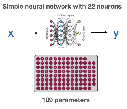
Even a relatively basic neural network with just 22 neurons can have over 100 parameters:

Now consider large-scale models used in natural language processing (like ChatGPT).
These models are massive, with a staggering number of parameters:

• GPT-3 (2020) has 175 billion parameters
• OpenAI has not published the size of its later models; unofficial estimates for GPT-4 (2023) are around 1.8 trillion parameters

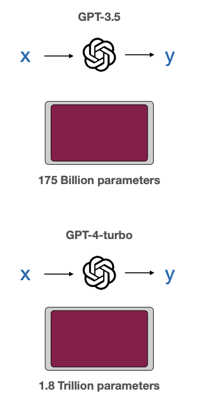
The labels in this figure (GPT-3.5, GPT-4 Turbo) follow figures that circulated online: 175 billion is the published size of GPT-3, and 1.8 trillion is an unofficial estimate for GPT-4.

The amount of data needed to estimate the parameters reliably grows very fast as the number of inputs and parameters grows. This is what the curse of dimensionality refers to. You met a small version of it in the exercise above, where one data point could not pin down four parameters.
It's one of the central challenges when working with AI models, especially in fields like sport science, where data may be limited or noisy.

Keep it in mind when you choose or design a model for performance prediction, injury prevention, or workload optimization.

How does a large language model (LLM) work?

Throughout this course, we've described models as services that take inputs (x) and produce outputs (y), with parameters adjusted to find the best fit. Large language models (LLMs) like ChatGPT work on the same principle, at a much larger scale.

Think of an LLM as a text prediction service. Just as our VO₂ model takes power as input and predicts oxygen consumption, an LLM takes text as input and predicts the next word that should come after it.

First, the text has to become numbers: each word is converted into a position in a high-dimensional mathematical space, which the model can process. What comes out is not a single word but a probability for each possible next word. After "The weather is...", "sunny" or "cloudy" might get a high probability and "bicycle" a low one.

In between sit the parameters. Our HR_max model had 2 of them, and the chicken growth example up to 5. GPT-3 has 175 billion: weights and biases like those in the neural network you trained by hand earlier, only far more of them.

Training works as in Module 2, where we minimized the RMSEM2. The model is shown huge amounts of text, and its parameters are adjusted until it gets better at predicting the next word. It is the same parameter estimation process we've used throughout, with far more data.

This is also why an LLM can seem "intelligent" without understanding language the way we do. By processing so much text, its parameters have captured detailed statistical patterns of how words tend to follow each other. When you ask ChatGPT "What's the best training method for VO₂max improvement?", it's not consulting a physiology textbook: it predicts, word by word, the text most likely to follow your question, based on the patterns it learned during training.

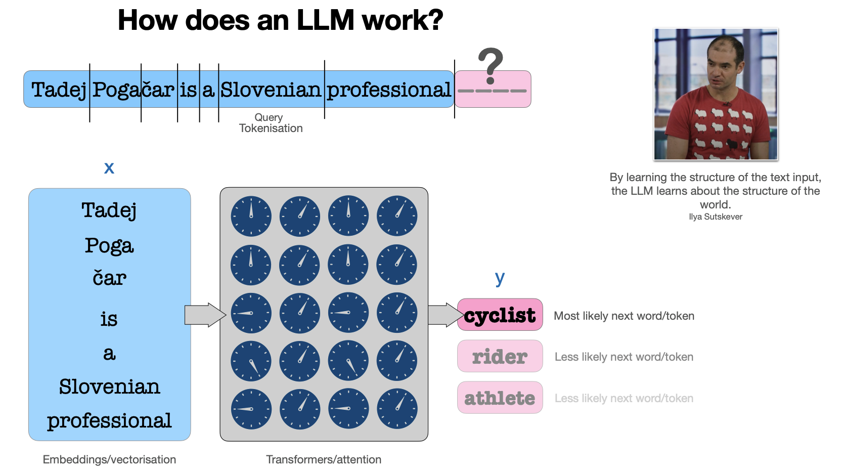
This is the same modeling approach we've used for heart rate prediction, lactate clearance, and power-duration curves, scaled up to handle human language. The core principle is unchanged: input → parameters → output, with optimization driving the learning.

Wrap-up

Well done, you have completed the fifth module of this course.